数据处理(numpy & pandas & scipy & matplotlib.pyplot)

2019-04-02 | 阅读：次

数据处理(numpy & pandas & scipy & matplotlib.pyplot)

numpy

参考网址： https://www.jianshu.com/p/57e3c0a92f3a 啥都解释了：https://zhuanlan.zhihu.com/p/20878530

小知识点

迭代对象与迭代器：https://blog.csdn.net/jinixin/article/details/72232604 my_list_iter = iter(my_list) # 得到该对象的迭代器实例，iter函数在下面会详细解释（iter获取迭代器。。。）
生成器是一种特殊的迭代器，生成器自动实现了“迭代器协议”（即__iter__和 next方法），不需要再手动实现两方法。
生成器在迭代的过程中可以改变当前迭代值，而修改普通迭代器的当前迭代值往往会发生异常，影响程序的执行。

#数学之美
import numpy as np
import matplotlib.pyplot as plt

def mandelbrot(h, w, maxit=20):
    y, x = np.ogrid[-1.4:1.4:h * 1j, -2:0.8:w * 1j]
    c = x + y * 1j
    z = c
    divtime = maxit + np.zeros(z.shape, dtype=int)
    for i in range(maxit):
        z = z ** 2 + c
        diverge = z * np.conj(z) > 2 ** 2  # who is diverging
        div_now = diverge & (divtime == maxit)  # who is diverging now
        divtime[div_now] = i  # note when
        z[diverge] = 2  # avoid diverging too much
    return divtime

plt.imshow(mandelbrot(400, 400))
plt.show()

柱形图 hist

import numpy as np
import matplotlib.pyplot as plt

# Build a vector of 10000 normal deviates with variance 0.5^2 and mean 2
mu, sigma = 2, 0.5
v = np.random.normal(mu, sigma, 10000)
# Plot a normalized histogram with 50 bins
plt.hist(v, bins=50, normed=1)  # matplotlib version (plot)
plt.show()

柱形图的顶点线型图

import numpy as np
import matplotlib.pyplot as plt

# Build a vector of 10000 normal deviates with variance 0.5^2 and mean 2
mu, sigma = 2, 0.5
v = np.random.normal(mu, sigma, 10000)
# Compute the histogram with numpy and then plot it
(n, bins) = np.histogram(v, bins=50, normed=True)  # NumPy version (no plot)
plt.plot(.5 * (bins[1:] + bins[:-1]), n)
plt.show()

合并：https://morvanzhou.github.io/tutorials/data-manipulation/np-pd/2-6-np-concat/

df2 = pd.DataFrame({'A' : 1.,
                    'B' : pd.Timestamp('20130102'),
                    'C' : pd.Series(1,index=list(range(4)),dtype='float32'),
                    'D' : np.array([3] * 4,dtype='int32'),
                    'E' : pd.Categorical(["test","train","test","train"]),
                    'F' : 'foo'})
                    
print(df2)

"""
     A          B    C  D      E    F
0  1.0 2013-01-02  1.0  3   test  foo
1  1.0 2013-01-02  1.0  3  train  foo
2  1.0 2013-01-02  1.0  3   test  foo
3  1.0 2013-01-02  1.0  3  train  foo
"""

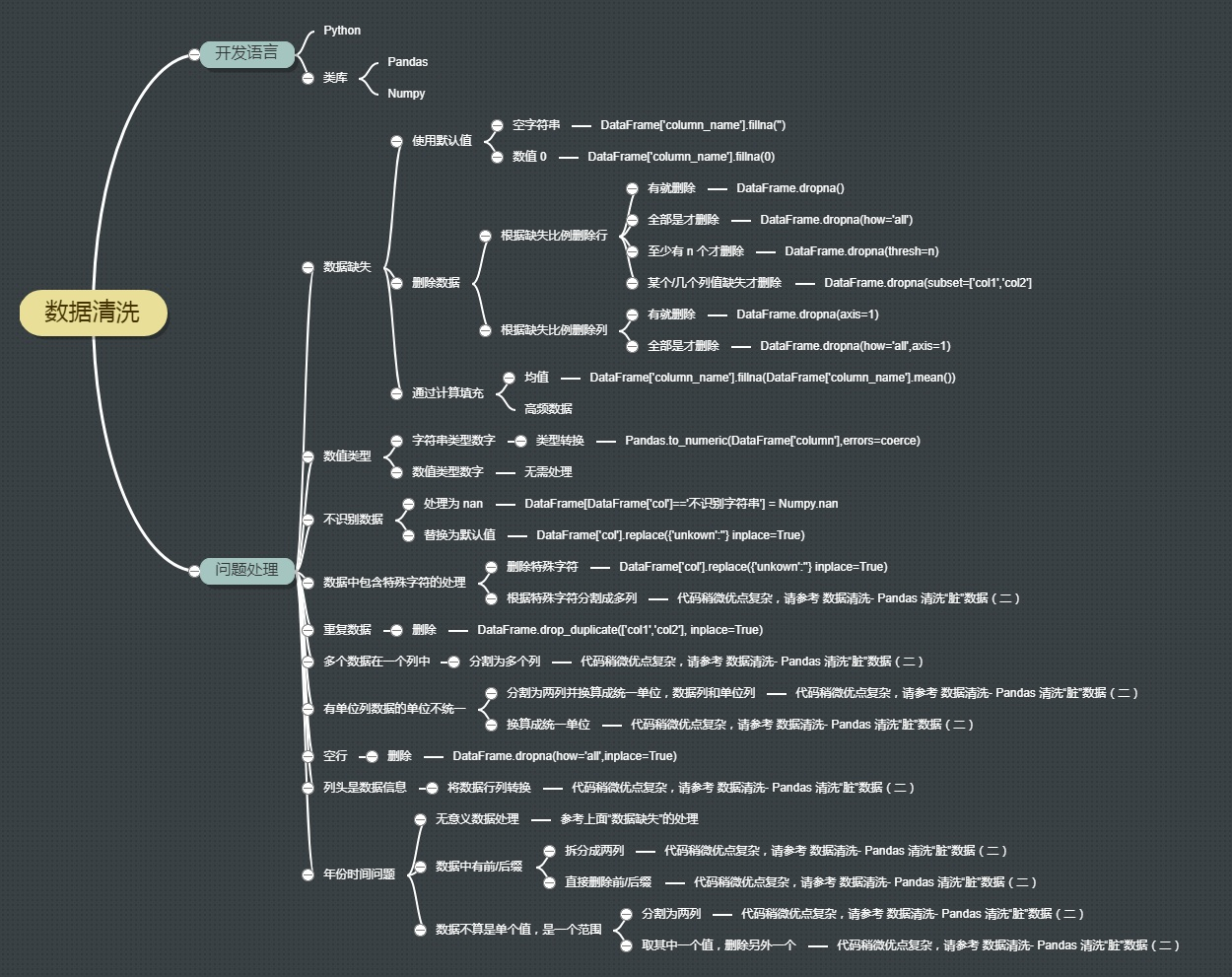
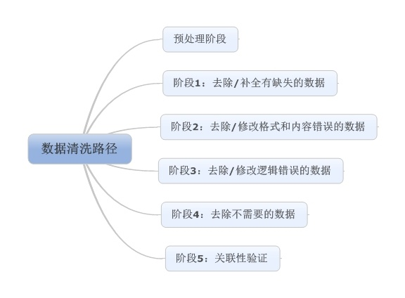
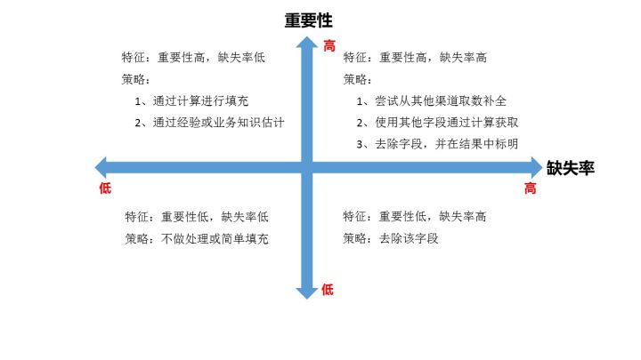
数据清洗

知乎专栏：https://zhuanlan.zhihu.com/dataclean

参考网址：https://zhuanlan.zhihu.com/p/20571505

pandas 小知识点学习参考

https://blog.csdn.net/tanzuozhev/column/info/16726

数据表中的重复值duplicated() & drop_duplicates()
数据表中的空值 isnull() & notnull() & fillna(0)–>填充nan为0 & dropna()

数据间的空格

loandata['term']=loandata['term'].map(str.strip)
loandata['term']=loandata['term'].map(str.lstrip)
loandata['term']=loandata['term'].map(str.rstrip)

大小写转换：

loandata['term']=loandata['term'].map(str.upper)
loandata['term']=loandata['term'].map(str.lower)
loandata['term']=loandata['term'].map(str.title)

数据清洗

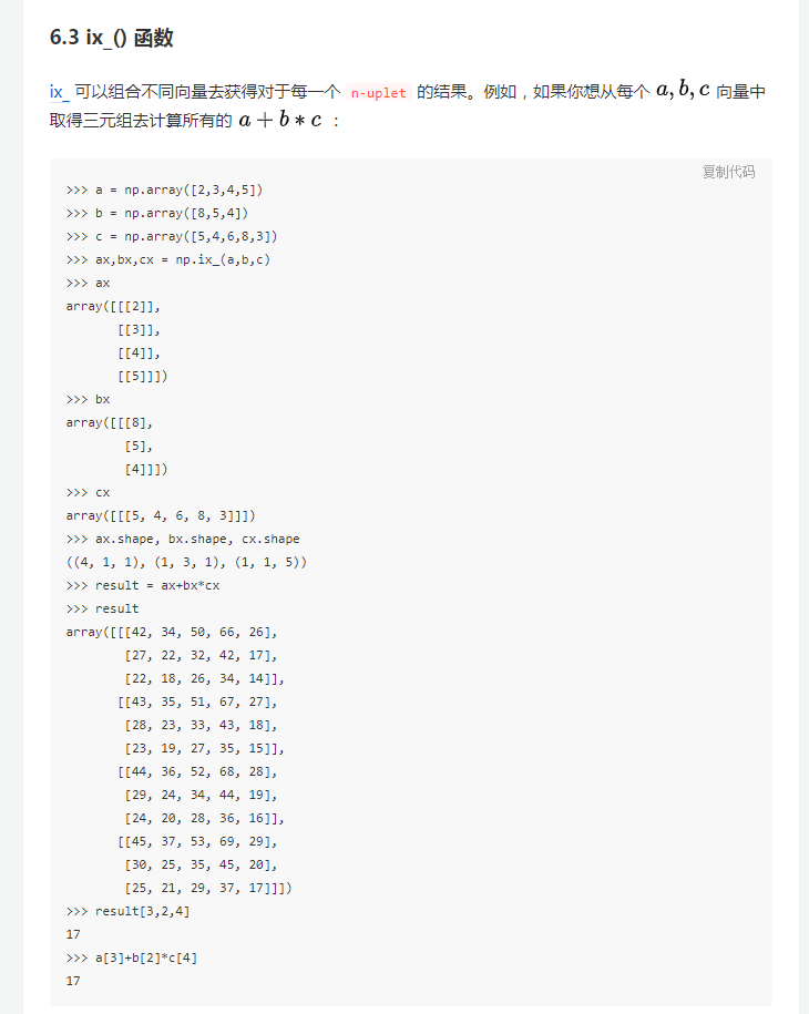
pandas中Dataframe的查询方法（[], loc, iloc, at, iat, ix）：https://blog.csdn.net/wr339988/article/details/65446138
pandas学习笔记5—DataFrame数据筛选loc，iloc，ix，at，iat：https://blog.csdn.net/liuweiyuxiang/article/details/78241530
https://segmentfault.com/a/1190000014117720
索引修改
正则清洗数据
删除 DataFrame 中的不必要 columns
改变 DataFrame 的 index
使用 .str() 方法来清洗 columns
使用 DataFrame.applymap() 函数按元素的清洗整个数据集
重命名 columns 为一组更易识别的标签
滤除 CSV文件中不必要的 rows
loc基于索引、iloc基于位置

Pandas透视表（pivot_table）详解

https://blog.csdn.net/liuweiyuxiang/article/details/78183896

inplace=True–>表示在原数据或者结构上进行操作修改

pandas的factorize()理解

factorize函数可以将Series中的标称型数据映射称为一组数字，相同的标称型映射为相同的数字。factorize函数的返回值是一个tuple（元组），元组中包含两个元素。第一个元素是一个array，其中的元素是标称型元素映射为的数字；第二个元素是Index类型，其中的元素是所有标称型元素，没有重复。

import numpy as np
import pandas as pd
In [43]: df = pd.DataFrame({"id":[1,2,3,4,5,6,3,2], "raw_grade":['a', 'b', 'b',
    ...:  'a', 'a', 'e','c','a']})

In [44]: df
Out[44]:
   id raw_grade
0   1         a
1   2         b
2   3         b
3   4         a
4   5         a
5   6         e
6   3         c
7   2         a

In [45]: x = pd.factorize(df.raw_grade)

In [46]: x
Out[46]:
(array([0, 1, 1, 0, 0, 2, 3, 0], dtype=int64),
 Index(['a', 'b', 'e', 'c'], dtype='object'))
#array中的元素其实是df.raw_grade的对应位置元素在Index中的下标。例如array第一个元素是0，表示df.raw_grade的第一个元素为Index的第0个元素。

In [47]: x[1]
Out[47]: Index(['a', 'b', 'e', 'c'], dtype='object')

In [48]: x[0]
Out[48]: array([0, 1, 1, 0, 0, 2, 3, 0], dtype=int64)

In [49]: type(x)
Out[49]: tuple

pandas 修改DataFrame列名

参考链接：https://blog.csdn.net/liuweiyuxiang/article/details/78445440

>>>a.rename(columns={'A':'a', 'B':'b', 'C':'c'}, inplace = True)
>>>a
   a  b  c
0  1  4  7
1  2  5  8
2  3  6  9

>>>a.rename(columns={'A':'a', 'C':'c'}, inplace = True) # inplace的意思是在原DataFrame上完成
>>>a
   a  B  c
0  1  4  7
1  2  5  8
2  3  6  9
# 可以只修改A，C两列的名称，而不修改B。

pandas 值的替换

replace_map={
    -999:None
}
obj.replace(replace_map)
||
frame.rename(
    index={'Ohio':'Indiana'},
    columns={'three':'peekaboo'},
    inplace=True
)

数据重排与随机采样

根据给定的索引对行进行重排，选取数据等。

frame=pd.DataFrame(np.arange(20).reshape((5,4)))
re_order=np.random.permutation(frame.shape[0])

training_set=frame.iloc[re_order[:3],:]
test_set=frame.iloc[re_order[3:],:]
mini_batch=training_set.sample(1,replace=True)

非 ASCII 字符

# 删除非 ASCII 字符
df['first_name'].replace({r'[^\x00-\x7F]+':''}, regex=True, inplace=True)
df['last_name'].replace({r'[^\x00-\x7F]+':''}, regex=True, inplace=True)

pandas中关于axis的理解

参考链接：https://blog.csdn.net/liuweiyuxiang/article/details/80895844

例如一个shape（3，2，4）的数组，代表一个三维数组，要注意的是这里的维度与物理学的维度的理解是不太一样的 axis = 0时，就相当于所求的数组的结果变成shape（2，4） axis = 1时，数组的结果shape（3，4） axis = 2时，数组的结果shape（3，2）这里应该看出来了，当axis=n的时候shape中相应的索引就会被去除，数组发生了降维，那么是如何降维的呢？首先要清楚shape里的数字都代表什么意义： 3代表这个numpy数组里嵌套着3个数组（有三层）， 2代表其中每个数组的行数，3代表其中每个数组的列数。

>>>df = pd.DataFrame([[1, 1, 1, 1], [2, 2, 2, 2], [3, 3, 3, 3]], \
columns=["col1", "col2", "col3", "col4"])
>>>df
   col1  col2  col3  col4
    0     1     1     1     1
    1     2     2     2     2
    2     3     3     3     3
# 如果我们调用df.mean(axis=1),我们将得到按行计算的均值
>>> df.mean(axis=1)
0    1
1    2
2    3
然而，如果我们调用 df.drop((name, axis=1),我们实际上删掉了一列，而不是一行：
>>> df.drop("col4", axis=1)
   col1  col2  col3
0     1     1     1
1     2     2     2
2     3     3     3

其实问题理解axis有问题，df.mean其实是在每一行上取所有列的均值，而不是保留每一列的均值。也许简单的来记就是axis=0代表往跨行（down)，而axis=1代表跨列（across)，作为方法动作的副词（译者注）

换句话说:

使用0值表示沿着每一列或行标签\索引值向下执行方法
使用1值表示沿着每一行或者列标签模向执行对应的方法

下图代表在DataFrame当中axis为0和1时分别代表的含义:

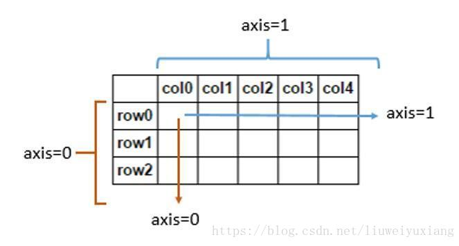
axis参数作用方向图示。另外，记住，Pandas保持了Numpy对关键字axis的用法，用法在Numpy库的词汇表当中有过解释：轴用来为超过一维的数组定义的属性，二维数据拥有两个轴：第0轴沿着行的垂直往下，第1轴沿着列的方向水平延伸。所以问题当中第一个列子 df.mean(axis=1)代表沿着列水平方向计算均值，而第二个列子df.drop(name, axis=1) 代表将name对应的列标签（们）沿着水平的方向依次删掉。即df.mean(axis=1)表示一行一行的计算均值，df.drop(name, axis=1)表示一行一行的将name列删掉。还可以这样理解，axis等于那个维度代表操作在哪个维度上进行，操作后该维度消失(变成1)。如df.mean(axis=1)，axis=1表示均值操作在列上进行(跨列操作)，即按照行相加求均值，操作后变成一列。axis指定哪个维度表示跨哪个维度进行操作。

scikit-learn中评估分类器性能的度量，像混淆矩阵、ROC、AUC等

参考链接：https://blog.csdn.net/liuweiyuxiang/article/details/78475419

数据处理常用函数大全

import numpy as np  
import pandas as pd  
import matplotlib.pyplot as plt
from pandas import read_csv;
from pandas import to_datetime;    
  
  
---------------numpy-----------------------  
arr = np.array([1,2,3], dtype=np.float64)  
np.zeros((3,6))  np.empty((2,3,2)) np.arange(15)  
arr.dtype arr.ndim arr.shape  
arr.astype(np.int32) #np.float64 np.string_ np.unicode_  
arr * arr arr - arr 1/arr  
arr= np.arange(32).reshape((8,4))  
arr[1:3, : ]  #正常切片  
arr[[1,2,3]]  #花式索引  
arr.T   arr.transpose((...))   arr.swapaxes(...) #转置  
arr.dot #矩阵内积  
np.sqrt(arr)   np.exp(arr)    randn(8)＃正态分布值   np.maximum(x,y)  
np.where(cond, xarr, yarr)  ＃当cond为真，取xarr,否则取yarr  
arr.mean()  arr.mean(axis=1)   #算术平均数  
arr.sum()   arr.std()  arr.var()   #和、标准差、方差  
arr.min()   arr.max()   #最小值、最大值  
arr.argmin()   arr.argmax()    #最小索引、最大索引  
arr.cumsum()    arr.cumprod()   #所有元素的累计和、累计积  
arr.all()   arr.any()   # 检查数组中是否全为真、部分为真  
arr.sort()   arr.sort(1)   #排序、1轴向上排序  
arr.unique()   #去重  
np.in1d(arr1, arr2)  #arr1的值是否在arr2中  
np.load() np.loadtxt() np.save() np.savez() ＃读取、保存文件  
np.concatenate([arr, arr], axis=1)  ＃连接两个arr，按行的方向  
  
  
---------------pandas-----------------------  
ser = Series()     ser = Series([...], index=[...])  #一维数组, 字典可以直接转化为series  
ser.values    ser.index    ser.reindex([...], fill_value=0)  #数组的值、数组的索引、重新定义索引  
ser.isnull()   pd.isnull(ser)   pd.notnull(ser)   #检测缺失数据  
ser.name=       ser.index.name=    #ser本身的名字、ser索引的名字  
ser.drop('x') #丢弃索引x对应的值  
ser +ser  #算术运算  
ser.sort_index()   ser.order()     ＃按索引排序、按值排序  
df = DataFrame(data, columns=[...], index=[...]) #表结构的数据结构，既有行索引又有列索引  
df.ix['x']  #索引为x的值    对于series，直接使用ser['x']  
del df['ly']  #用del删除第ly列  
df.T    #转置  
df.index.name df.columns.name df.values  
df.drop([...])  
df + df   df1.add(df2, fill_vaule=0) #算术运算  
df -ser   #df与ser的算术运算  
f=lambda x: x.max()-x.min()   df.apply(f)  
df.sort_index(axis=1, ascending=False)   #按行索引排序  
df.sort_index(by=['a','b'])   #按a、b列索引排序  
ser.rank()   df.rank(axis=1)  #排序，增设一个排名值  
df.sum()   df.sum(axis=1)   #按列、按行求和  
df.mean(axis=1, skipna=False)   #求各行的平均值，考虑na的存在  
df.idxmax()   #返回最大值的索引  
df.cumsum()   #累计求和  
df.describe()  ser.describe()   #返回count mean std min max等值  
ser.unique()  #去重  
ser.value_counts()   df.value_counts()  ＃返回一个series，其索引为唯一值，值为频率  
ser.isin(['x', 'y'])  #判断ser的值是否为x,y，得到布尔值  
ser.dropna() ser.isnull() ser.notnull() ser.fillna(0)  #处理缺失数据，df相同  
df.unstack()   #行列索引和值互换  df.unstack().stack()  
df.swaplevel('key1','key2')   #接受两个级别编号或名称，并互换  
df.sortlevel(1) #根据级别1进行排序，df的行、列索引可以有两级  
df.set_index(['c','d'], drop=False)    #将c、d两列转换为行,因drop为false，在列中仍保留c,d  
read_csv   read_table   read_fwf    #读取文件分隔符为逗号、分隔符为制表符('\t')、无分隔符（固定列宽）  
pd.read_csv('...', nrows=5) #读取文件前5行  
pd.read_csv('...', chunksize=1000) #按块读取，避免过大的文件占用内存  
pd.load() #pd也有load方法，用来读取二进制文件  
pd.ExcelFile('...xls').parse('Sheet1')  # 读取excel文件中的sheet1  
df.to_csv('...csv', sep='|', index=False, header=False) #将数据写入csv文件，以｜为分隔符，默认以，为分隔符, 禁用列、行的标签  
pd.merge(df1, df2, on='key', suffixes=('_left', '_right')) #合并两个数据集,类似数据库的inner join, 以二者共有的key列作为键,suffixes将两个key分别命名为key_left、key_right  
pd.merge(df1, df2, left_on='lkey', right_on='rkey') #合并，类似数据库的inner join, 但二者没有同样的列名，分别指出，作为合并的参照  
pd.merge(df1, df2, how='outer') #合并，但是是outer join；how='left'是笛卡尔积，how='inner'是...;还可以对多个键进行合并  
df1.join(df2, on='key', how='outer')  #也是合并  
pd.concat([ser1, ser2, ser3], axis=1) #连接三个序列，按行的方向  
ser1.combine_first(ser2)   df1.combine_first(df2) #把2合并到1上，并对齐  
df.stack() df.unstack()  #列旋转为行、行旋转为列  
df.pivot()  
df.duplicated()   df.drop_duplicates() #判断是否为重复数据、删除重复数据  
df[''].map(lambda x: abs(x)) #将函数映射到df的指定列  
ser.replace(-999, np.nan) #将－999全部替换为nan  
df.rename(index={}, columns={}, inplace=True) #修改索引，inplace为真表示就地修改数据集  
pd.cut(ser, bins)  #根据面元bin判断ser的各个数据属于哪一个区段，有labels、levels属性  
df[(np.abs(df)>3).any(1)] #输出含有“超过3或－3的值”的行  
permutation  take    #用来进行随机重排序  
pd.get_dummies(df['key'], prefix='key')  #给df的所有列索引加前缀key  
df[...].str.contains()  df[...].str.findall(pattern, flags=re.IGNORECASE)  df[...].str.match(pattern, flags=...)    df[...].str.get()  #矢量化的字符串函数  
  
----绘图  
ser.plot() df.plot() #pandas的绘图工具，有参数label, ax, style, alpha, kind, logy, use_index, rot, xticks, xlim, grid等，详见page257  
kind='kde' #密度图  
kind='bar' kind='barh' #垂直柱状图、水平柱状图，stacked=True为堆积图  
ser.hist(bins=50) #直方图  
plt.scatter(x,y) #绘制x,y组成的散点图  
pd.scatter_matrix(df, diagonal='kde', color='k', alpha='0.3')  #将df各列分别组合绘制散点图  
  
----聚合分组  
groupby() 默认在axis=0轴上分组，也可以在1组上分组；可以用for进行分组迭代  
df.groupby(df['key1']) #根据key1对df进行分组  
df['key2'].groupby(df['key1'])  #根据key1对key2列进行分组  
df['key3'].groupby(df['key1'], df['key2'])  #先根据key1、再根据key2对key3列进行分组  
df['key2'].groupby(df['key1']).size() #size()返回一个含有分组大小的series  
df.groupby(df['key1'])['data1']  等价于 df['data1'].groupby(df['key1'])  
df.groupby(df['key1'])[['data1']]  等价于  df[['data1']].groupby(df['key1'])  
df.groupby(mapping, axis=1)  ser(mapping) #定义mapping字典，根据字典的分组来进行分组  
df.groupby(len) #通过函数来进行分组，如根据len函数  
df.groupby(level='...', axis=1)  #根据索引级别来分组  
df.groupby([], as_index=False)   #禁用索引，返回无索引形式的数据  
df.groupby(...).agg(['mean', 'std'])   #一次使用多个聚合函数时，用agg方法  
df.groupby(...).transform(np.mean)   #transform()可以将其内的函数用于各个分组  
df.groupby().apply()  #apply方法会将待处理的对象拆分成多个片段，然后对各片段调用传入的函数，最后尝试将各片段组合到一起  
  
----透视交叉  
df.pivot_table(['',''], rows=['',''], cols='', margins=True)  #margins为真时会加一列all  
pd.crosstab(df.col1, df.col2, margins=True) #margins作用同上  
  
  
---------------matplotlib---------------  
fig=plt.figure() ＃图像所在的基对象  
ax=fig.add_subplot(2,2,1)  #2*2的图像，当前选中第1个  
fig, axes = plt.subplots(nrows, nclos, sharex, sharey)  #创建图像，指定行、列、共享x轴刻度、共享y轴刻度  
plt.subplots_adjust(left=None, bottom=None, right=None, top=None, wspace=None, hspace=None)  
#调整subplot之间的距离，wspace、hspace用来控制宽度、高度百分比  
ax.plot(x, y, linestyle='--', color='g')   #依据x,y坐标画图，设置线型、颜色  
ax.set_xticks([...]) ax.set_xticklabels([...]) #设置x轴刻度  
ax.set_xlabel('...') #设置x轴名称  
ax.set_title('....') ＃设置图名  
ax.legend(loc='best') #设置图例， loc指定将图例放在合适的位置  
ax.text(x,y, 'hello', family='monospace', fontsize=10) #将注释hello放在x,y处，字体大小为10  
ax.add_patch() #在图中添加块  
plt.savefig('...png', dpi=400, bbox_inches='tight') #保存图片，dpi为分辨率，bbox＝tight表示将裁减空白部分  
  
  
  
  
------------------------------------------  
from mpl_toolkits.basemap import Basemap  
import matplotlib.pyplot as plt  
#可以用来绘制地图  
  
  
-----------------时间序列--------------------------  
pd.to_datetime(datestrs)    #将字符串型日期解析为日期格式  
pd.date_range('1/1/2000', periods=1000)    #生成时间序列  
ts.resample('D', how='mean')   #采样，将时间序列转换成以每天为固定频率的, 并计算均值；how='ohlc'是股票四个指数；  
＃重采样会聚合，即将短频率（日）变成长频率（月），对应的值叠加；  
＃升采样会插值，即将长频率变为短频率，中间产生新值  
ts.shift(2, freq='D')   ts.shift(-2, freq='D') #后移、前移2天  
now+Day() now+MonthEnd()  
import pytz   pytz.timezone('US/Eastern')   #时区操作，需要安装pytz  
pd.Period('2010', freq='A-DEC')   ＃period表示时间区间，叫做时期  
pd.PeriodIndex    #时期索引  
ts.to_period('M')   #时间转换为时期  
pd.rolling_mean(...)    pd.rolling_std(...)   #移动窗口函数－平均值、标准差 
df = read_csv('D:\\PA\\4.18\\data.csv', encoding='utf8')
df_dt = to_datetime(df.注册时间, format='%Y/%m/%d');
df_dt.dt.year
df_dt.dt.second;
df_dt.dt.minute;
df_dt.dt.hour;
df_dt.dt.day;
df_dt.dt.month;
df_dt.dt.weekday;

处理丢失数据

df.dropna(
    axis=0,     # 0: 对行进行操作; 1: 对列进行操作
    how='any'   # 'any': 只要存在 NaN 就 drop 掉; 'all': 必须全部是 NaN 才 drop 
    ) 
df.fillna(value=0)
df.isnull() # 得到的是布尔型的矩阵
np.any(df.isnull()) == True  # 判断是否存在Nan

导入导出数据

import pandas as pd #加载模块

#读取csv
data = pd.read_csv('student.csv')

#打印出data
print(data)
data.to_pickle('student.pickle') # 将资料存取成pickle

ZoE

ZoE

数据处理(numpy & pandas & scipy & matplotlib.pyplot)